Mapping buildings by construction year (BAG)
Source:vignettes/articles/bag-buildings.Rmd
bag-buildings.RmdThe BAG (Basisregistratie Adressen
en Gebouwen) holds every building in the Netherlands, with attributes
such as the year it was built. It is served over the OGC API Features
service, so pdok_read() reads it like any other layer. This
article maps the buildings of one neighborhood, colored by construction
year.
library(pdokr)
library(tmap)
library(dplyr)
#>
#> Attaching package: 'dplyr'
#> The following objects are masked from 'package:stats':
#>
#>     filter, lag
#> The following objects are masked from 'package:base':
#>
#>     intersect, setdiff, setequal, union
Choose an area
We use the administrative boundaries to select the
Stadsdriehoek, the historic center of Rotterdam.
gemeenten <- pdok_read(
  "cbs/gebiedsindelingen", "gemeente_gegeneraliseerd", datetime = 2025
)
rotterdam <- filter(gemeenten, statnaam == "Rotterdam")

buurten <- pdok_read(
  "cbs/gebiedsindelingen", "buurt_gegeneraliseerd", datetime = 2025,
  filter_by = rotterdam, predicate = "within"
)
stadsdriehoek <- filter(buurten, statnaam == "Stadsdriehoek")
Load every building in it
The kadaster/bag dataset has a pand
(building) layer. We filter it to the neighborhood;
pdok_read() pre-filters at the server and clips to the
exact shape.
buildings <- pdok_read("kadaster/bag", "pand", filter_by = stadsdriehoek)
#> ⠙ Downloading PDOK features: 363 fetched
#> ⠹ Downloading PDOK features: 808 fetched
#> ⠹ Downloading PDOK features: 1022 fetched
nrow(buildings)
#> [1] 1022
BAG records an unknown construction year as 9999; we set
those to NA.
Map by construction year
Rotterdam’s historic center was largely destroyed in the May 1940 bombing and rebuilt afterwards. To make that dividing line jump out, we color the buildings that pre-date the bombing (before 1940) in cool blues and the post-war rebuild in warm tones — the surviving pre-war buildings stand out against a sea of reconstruction.
tmap_mode("plot")
#> ℹ tmap modes "plot" - "view"
#> ℹ toggle with `tmap::ttm()`

era_scale <- tm_scale_intervals(
  breaks = c(1600, 1900, 1940, 1960, 1980, 2000, 2026),
  values = c("#1f78b4", "#a6cee3", "#ffffb2", "#fecc5c", "#fd8d3c", "#e31a1c"),
  # Years are not thousands: drop the "." group separator (1.900 -> 1900).
  label.format = tm_label_format(big.mark = "")
)

tm_basemap(pdok_basemap("grijs")) +
  tm_shape(buildings) +
  tm_polygons(fill = "bouwjaar", fill.scale = era_scale, col = NULL) +
  tm_title("Buildings in Rotterdam's Stadsdriehoek, by construction year") +
  tm_credits("Kaartgegevens © Kadaster")
#> [plot mode] fit legend/component: Some legend items or map compoments do not
#> fit well, and are therefore rescaled.
#> ℹ Set the tmap option `component.autoscale = FALSE` to disable rescaling.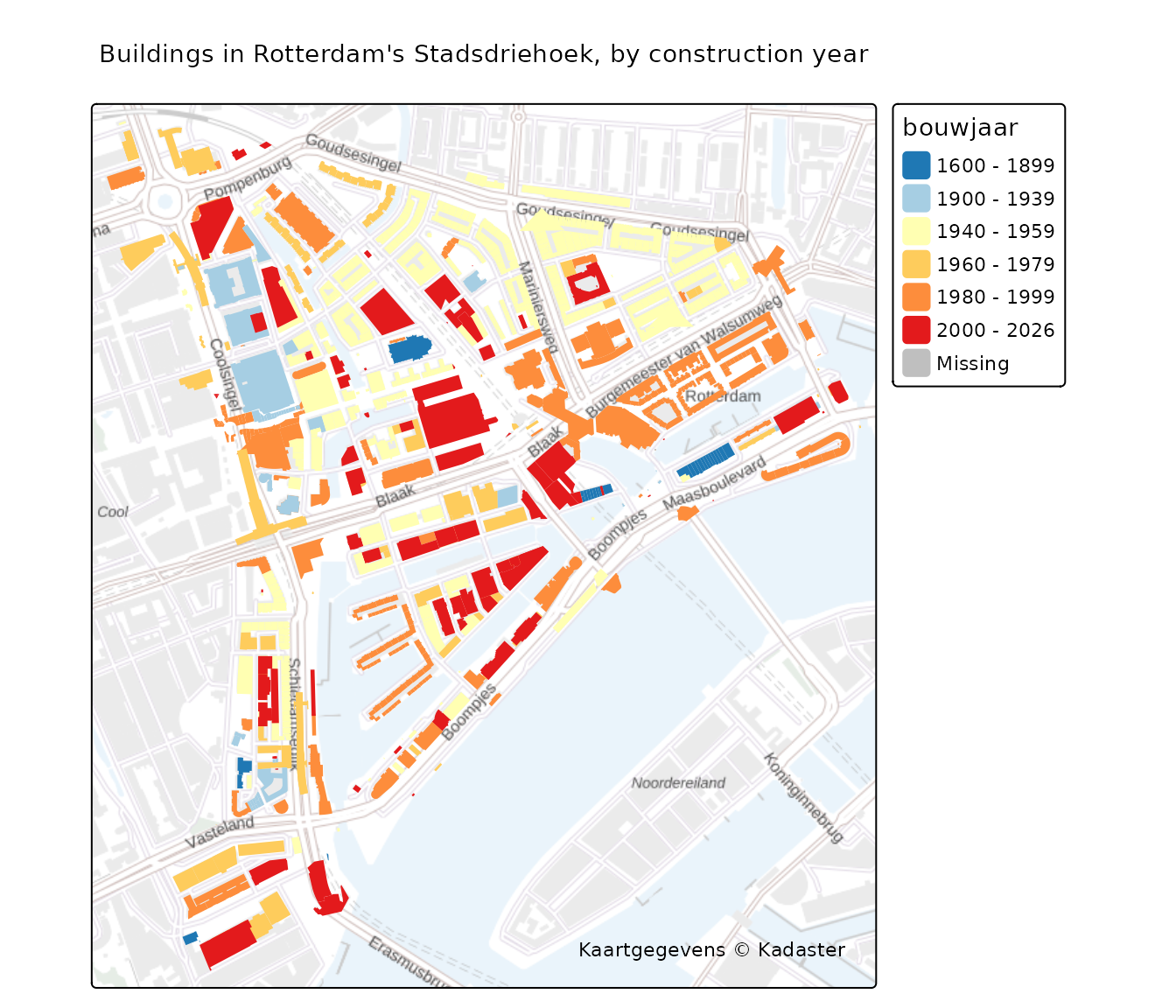
The same map interactively — zoom in and click a building:
tmap_mode("view")
#> ℹ tmap modes "plot" - "view"

tm_basemap(pdok_basemap("grijs")) +
  tm_shape(buildings) +
  tm_polygons(fill = "bouwjaar", fill.scale = era_scale, col = NULL,
              id = "identificatie",
              popup = tm_popup(vars = c("Built" = "bouwjaar"),
                               format = tm_label_format(big.mark = ""))) +
  tm_credits("Kaartgegevens © Kadaster")
Where to next
- Filtering data by area — the load-then-filter workflow used here.
-
Combining with external data — join
pdokrwith another open API. - PDOK basemaps — the gray background map used here, and the other styles.