Statistics Netherlands (CBS)
publishes a yearly dataset with hundreds of figures per neighborhood —
population, income, housing, energy use, distance to amenities, and much
more. Because PDOK serves it with geometry, a single
pdok_read() gives you everything you need for a choropleth.
This article maps the population density across the neighborhoods of
Amsterdam.
library(pdokr)
library(tmap)
library(dplyr)
#>
#> Attaching package: 'dplyr'
#> The following objects are masked from 'package:stats':
#>
#>     filter, lag
#> The following objects are masked from 'package:base':
#>
#>     intersect, setdiff, setequal, union
Read the neighborhoods of one municipality
The cbs/wijken-en-buurten-2025 dataset has
gemeenten, wijken and buurten
layers. We take the boundary of Amsterdam from the
gemeenten layer, then read the buurten
(neighborhoods) inside it.
gemeenten <- pdok_read("cbs/wijken-en-buurten-2025", "gemeenten")
#> ⠙ Downloading PDOK features: 424 fetched
amsterdam <- filter(gemeenten, gemeentenaam == "Amsterdam")

buurten <- pdok_read(
  "cbs/wijken-en-buurten-2025", "buurten",
  filter_by = amsterdam, predicate = "within"
)
#> ⠙ Downloading PDOK features: 519 fetched
nrow(buurten)
#> [1] 519
Handle the “no data” code
CBS marks a figure that is unknown or suppressed (too few cases, or a
non-residential area) with a large negative sentinel such as
-99997. We turn those into NA so they do not
distort the map.
buurten <- buurten |>
  mutate(bevolkingsdichtheid_inwoners_per_km2 =
           if_else(bevolkingsdichtheid_inwoners_per_km2 < 0, NA_real_,
                   bevolkingsdichtheid_inwoners_per_km2))
summary(buurten$bevolkingsdichtheid_inwoners_per_km2)
#>    Min. 1st Qu.  Median    Mean 3rd Qu.    Max.     NAs
#>       3    5689   10396   11815   17892   34968      44
The value is the number of inhabitants per square kilometer.
Draw the choropleth
A quantile classification keeps each color class roughly equal in size, which works well for a skewed variable like density. Neighborhoods without a value (water, parks, industry) are drawn in gray.
tmap_mode("plot")
#> ℹ tmap modes "plot" - "view"
#> ℹ toggle with `tmap::ttm()`

tm_basemap(pdok_basemap("grijs")) +
  tm_shape(buurten) +
  tm_polygons(
    fill = "bevolkingsdichtheid_inwoners_per_km2",
    fill.scale = tm_scale_intervals(n = 6, style = "quantile",
                                    values = "brewer.yl_or_rd"),
    fill.legend = tm_legend("Inhabitants per km2"),
    col = "white", lwd = 0.2, fill_alpha = 0.8
  ) +
  tm_title("Population density by neighborhood, Amsterdam (CBS 2025)") +
  tm_credits("Kaartgegevens © Kadaster")
#> [plot mode] fit legend/component: Some legend items or map compoments do not
#> fit well, and are therefore rescaled.
#> ℹ Set the tmap option `component.autoscale = FALSE` to disable rescaling.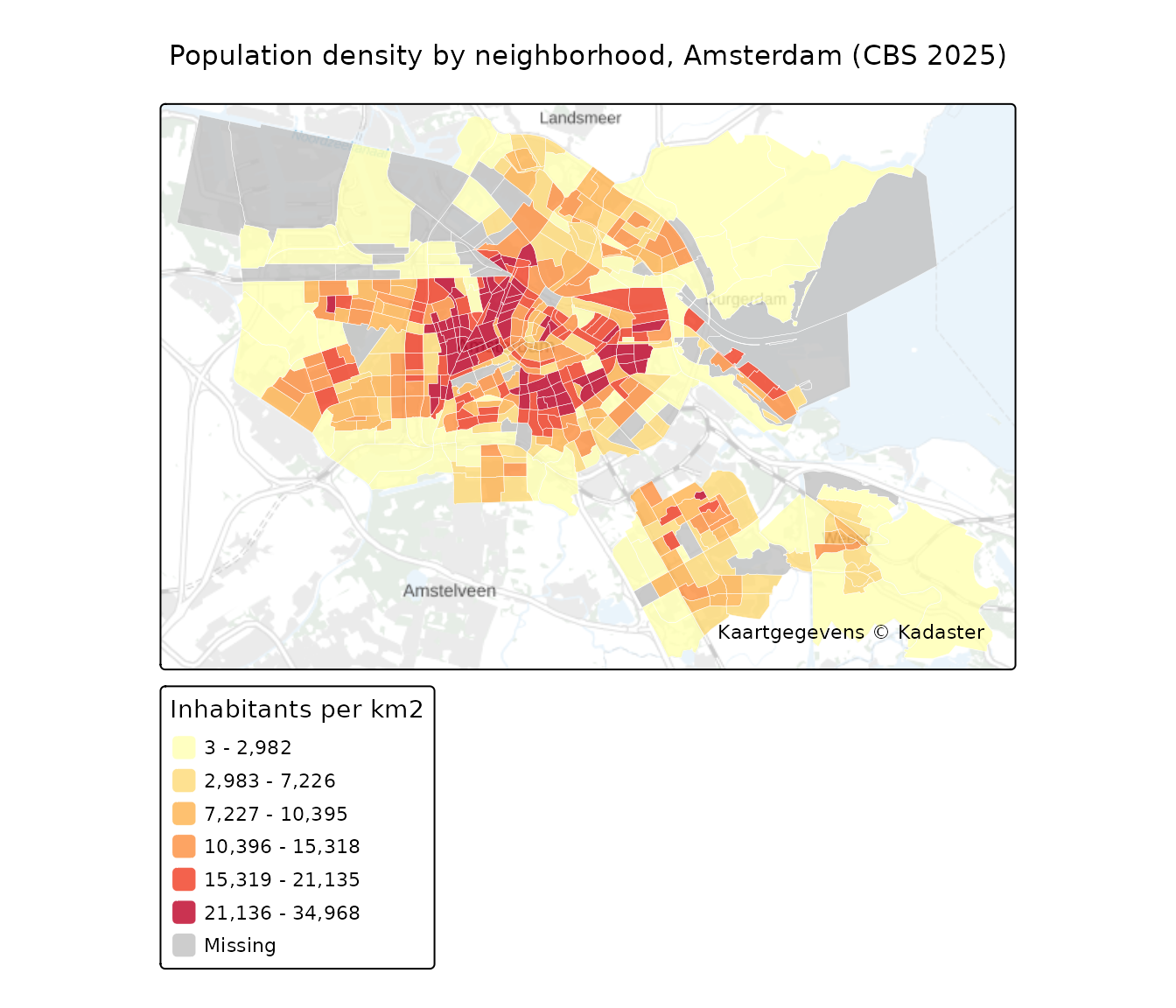
The same map interactively — hover for the neighborhood name and click for the value. A little transparency lets the basemap show through, so you keep your bearings:
tmap_mode("view")
#> ℹ tmap modes "plot" - "view"

tm_basemap(pdok_basemap("grijs")) +
  tm_shape(buurten) +
  tm_polygons(
    fill = "bevolkingsdichtheid_inwoners_per_km2",
    fill.scale = tm_scale_intervals(n = 6, style = "quantile",
                                    values = "brewer.yl_or_rd"),
    fill.legend = tm_legend("Inhabitants per km2"),
    col = "white", lwd = 0.2, fill_alpha = 0.6,
    id = "buurtnaam",
    popup = tm_popup(vars = c("Inhabitants per km2" = "bevolkingsdichtheid_inwoners_per_km2"))
  ) +
  tm_credits("Kaartgegevens © Kadaster")
To map a different figure, swap
bevolkingsdichtheid_inwoners_per_km2 for another column —
aantal_inwoners,
stedelijkheid_adressen_per_km2, or
gemiddelde_woningwaarde, among hundreds of others (some
figures appear a year or two after the boundaries).
Where to next
- Filtering data by area — the load-then-filter workflow.
- Coordinate reference systems — working in RD New (EPSG:28992), the Dutch national grid.
- PDOK basemaps — the gray background map used here, and the other styles.